Language Log

Fun with co-voting percentages

[Warning: significant geekery ahead. But those who like this sort of thing will find it just the sort of thing that they like.] I'm at CMU for a workshop on approaches to the analysis of U.S. Supreme Court oral arguments. This comes out of an NSF-funded research project that aims to take the tapes and transcripts from the shelves of the National Archives, and turn them into an on-line resource accessible to the public -- and also to scientists. The group doing this includes Jerry Goldman (a political scientist who is the proprietor of the oyez.org web site at Northwestern), Brian MacWhinney (a psychologist who runs the CHILDES and TalkBank sites), Tim Johnson (a political scientist from the University of Minnesota), and me, along with others at our various institutions. We've made quite a bit of progress towards the goal, and the purpose of this workshop is to engage some of our fellow scientists and scholars in thinking about how to use the data in research, as more and more of it becomes available, in more and more usable forms. The participants are a wide range of interesting people of all kinds, from legal scholars to psychologists, computer scientists, speech pathologists and sociolinguists (including my fellow Language Logger Roger Shuy!)

At some point in this morning's discussion, Tim Johnson mentioned the historical records of how various justices voted on various cases. I wondered whether anyone had analyzed such data using multi-dimensional scaling or similar techniques; and Jason Czarnezki mentioned some work by Peter Hook, recently discussed on the Empirical Legal Studies blog, that used a "spring force algorithm" to create a spatial arrangement of justices, based on mapping higher cumulative co-voting percentages to stronger springs. This isn't exactly the same thing, though it's conceptually similar -- perhaps someone has tried MDS on this problem as well, I don't know. So Jason also sent me a link to a paper in the Harvard Law Review ("Nine Justices ten years: a statistical retrospective", 118(1), November 2004), which presented exactly the sort of matrix needed to try it:

So I typed in the percentages:

100 51.0 81.3 78.0 84.9 63.8 79.4 63.2 63.0
51.0 100 57.0 44.3 58.7 76.2 45.3 78.0 75.6
81.3 57.0 100 70.2 78.5 71.3 70.4 66.1 71.6
78.0 44.3 70.2 100 72.9 55.4 86.7 53.5 51.7
84.9 58.7 78.5 72.9 100 67.9 73.7 66.7 65.6
63.8 76.2 71.3 55.4 67.9 100 54.1 85.6 81.5
79.4 45.3 70.4 86.7 73.7 54.1 100 52.2 51.0
63.2 78.0 66.1 53.5 66.7 85.6 52.2 100 82.1
63.0 75.6 71.6 51.7 65.6 81.5 51.0 82.1 100

And wrote a little R script to try Joe Kruskal's isoMDS algorithm:

Justices <- c("Rehnquist", "Stevens", "O'Connor", "Scalia", 
              "Kennedy", "Souter", "Thomas", "Ginsburg", "Breyer")
 Colors <- c("red", "black", "darkblue", "chocolate",
             "orange", "brown", "seagreen", "tomato1", "olivedrab")
 A <- read.table("SCOTUS.txt") # the table above...
 D <- 1.0 - A/100
 R <- isoMDS(as.dist(D), trace=T)
 xrange <- range(R$points[,1])
 yrange <- range(R$points[,2])
 xinc <- .1*(xrange[2]-xrange[1]); xrange[1] <- xrange[1]-xinc; xrange[2] <- xrange[2]+xinc
 #png(filename="Justices.png", width=700, height=700)
 plot(R$points[,1], R$points[,2], 
 xlab="Dimension 1", ylab="Dimension 2", xlim=xrange, type="n")
 text(R$points[,1], R$points[,2], labels=Justices, col=Colors)
 

The result:

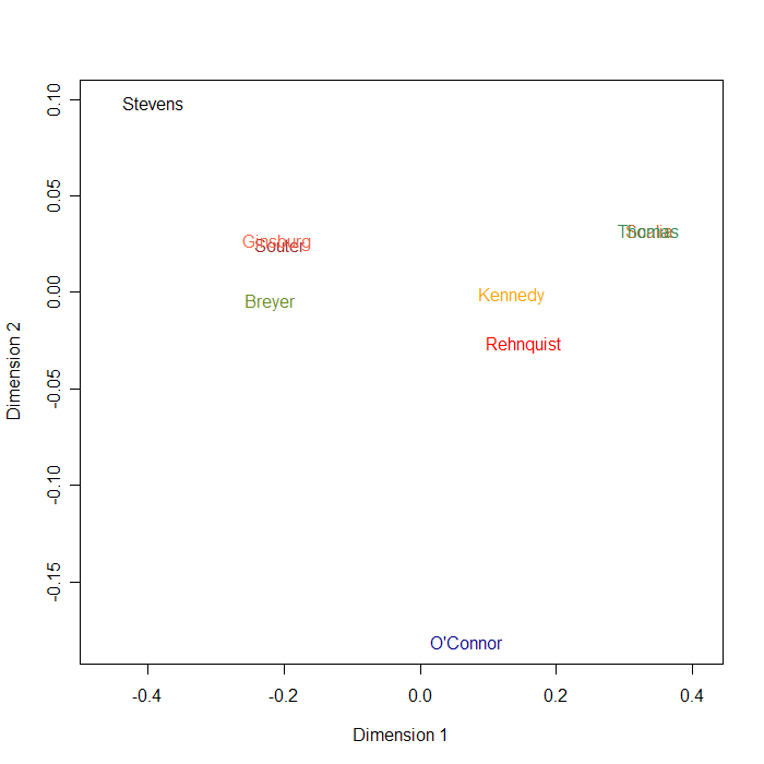
(The superimposed pair in the upper right of the plot is Scalia and Thomas.)

I guess this layout is a reasonable one.

Of course, that's the trouble with techniques like this -- usually, either they show you something that you already knew, or they show you something that doesn't make any sense. Still, this was easy and fun. It's not linguistics, but I guess it's the sort of thing that you might be able to use as part of a system for trying to understand what's going on in an argument.

[Update -- Fernando Pereira writes:

I thought that a log transform might work better, since "distances" in frequency space are best thought of as log or log ratios (cf. KL divergence). Result attached. As you commented, these things are best to confirm one's prejudices ;)

If you're singing along at home, just substitute:

D <- -log(A/100)
R <- isoMDS(as.dist(D), trace=T)

]

Posted by Mark Liberman at December 1, 2006 02:49 PM